A modern guide to SQL JOINs
Author: Alexey Makhotkin squadette@gmail.com, (~8800 words)
There are many SQL JOINs guides and tutorials, but this one takes a very different approach. Specifically:
-
LEFT JOIN is presented first, INNER JOIN second;
-
strict discipline of using ID equality comparison in ON condition;
-
we distinguish between N:1, 1:N and M:N cases of JOINs, with N:1 strictly preferred;
-
we avoid misleading wording and imagery;
-
we show a detailed explanation of overcounting in GROUP BY queries;
This guide will:
-
teach you how to write correct and fast SQL queries using JOINs;
-
show how to detect and fix problematic patterns in existing queries;
-
build a mental model that scales with the complexity of your queries;
Table of contents
Subscribe here to receive updates.
Prerequisites
You need a basic understanding of basic SQL. You may have read something about JOINs: tutorials, textbooks, watched some Youtube videos or whatever, but you feel that you don’t have a good understanding. This text is aimed at fixing your understanding by clarifying your mental model.
The goal of each section is to give you something surprising or enlightening. I’m not sure if that goal has always been achieved.
Table and data definitions and all SQL queries are here: https://dbfiddle.uk/GsdTPSed.
This text is generally applicable to any modern relational database.
Starting with LEFT JOIN
Use canonical syntax
Historically, there are many variations of SQL syntax. Generally speaking, you need to know various dialects to be able to read existing code that you may encounter. But here we’re going to primarily use a canonical simple syntax. This makes it easier to understand the meaning of different queries.
For LEFT JOIN we’re going to use a standard syntax:
SELECT tableA.*, tableB.*
FROM tableA LEFT JOIN tableB ON tableA.id = tableB.another_id
WHERE …
Here we have two different tables, called “tableA” and “tableB”.
tableA goes first, tableB goes second: table order is important.
“ON tableA.id = tableB.another_id” is called “ON condition”; it is
different from “WHERE condition”.
Use only ID equality in ON condition
Generally speaking, ON condition can be arbitrary (maybe even more than you thought, see below). We’ll discuss the full range of ON conditions in the second half of this chapter.
Here we’re going to primarily use a restricted case of ON conditions: ID equality. Getting back to our abstract example above:
SELECT tableA.*, tableB.*
FROM tableA LEFT JOIN tableB ON tableA.id = tableB.another_id
WHERE …
Look at the ON condition: it is a simple equality of two IDs: one from the first table, another from the second table.
Any other conditions, if needed, go into WHERE condition.
Why do we insist on that restriction? Virtually all practical SQL queries could be structured in this way. Moreover, later we’ll show how deviations from this discipline can lead to bugs. Don’t worry, we’ll have some fun by discussing some truly exotic ON conditions later in part 4.
“Learning foreign language” metaphor
When you learn a foreign language, there is an inherent asymmetry in what you can read and hear vs what you would write and say.
You can learn a relatively smaller number of words and expressions to say what you want. But other people could use different words and expressions even for the same concepts.
To understand them, you need to learn some words and expressions that you won’t even be using yourself. You can always use “thank you”, but eventually you need to learn that “much obliged” also means expressing gratitude.
Same with SQL (and other programming languages). You need to understand syntax variations, SQL dialects, different ways of designing tables, etc.
In this text we present a very disciplined way of writing SQL queries. We discuss other ways that are technically valid but may be confusing.
Unfortunately, it’s impossible to fully cover all variations. Some queries that you will encounter will genuinely be hard to read and understand, this is just a fact of life.
Example dataset: employees/payments
To demonstrate all the cases we want to discuss, we’re going to use a single tiny database consisting of two tables. In our imaginary scenario, we employ some people and we pay them money more or less regularly. Employees could be either full-time or contractors. Payments could be either salary or bonus. For people, we have names; for payments: amount and date. Additionally, some people are managers to other people, hierarchically. Finally, sometimes we send some payments to other companies, so payments.employee_id could be NULL.
Here is a straightforward table design:
CREATE TABLE people (
  id INTEGER NOT NULL PRIMARY KEY,
  name VARCHAR(64) NOT NULL,
  type VARCHAR(16) NOT NULL,
  manager_id INTEGER NULL
);

CREATE INDEX ndx_manager_id ON people(manager_id);

CREATE TABLE payments (
  id INTEGER NOT NULL PRIMARY KEY,
  employee_id INTEGER NULL,
  type VARCHAR(16) NOT NULL,
  amount INTEGER NOT NULL,
  date DATE NOT NULL,
  description VARCHAR(64) NOT NULL
);

CREATE INDEX ndx_employee_id ON payments(employee_id);
We also need to insert some representative data that covers all the patterns that we want to demonstrate. Let’s have five people, both full-time employees and contractors. Also, some of them are managers.
id |
name |
type |
manager_id |
|---|---|---|---|
| 1 | Alice | fulltime | NULL |
| 2 | Bob | fulltime | 1 |
| 3 | Carol | contractor | 2 |
| 4 | David | contractor | 1 |
| 5 | Eugene | fulltime | 2 |
As for payments, we need a different number of payments for each person, including zero. Also, we need payments of both types: bonus and salary. Also, we have one payment that is not directed to an employee.
| id | employee_id | type | amount | date | description |
|---|---|---|---|---|---|
| 1 | 1 | salary | 2000 | 2025-01-25 | Salary Jan 2025 |
| 2 | 1 | bonus | 1000 | 2025-02-10 | Bonus 2024 |
| 3 | 1 | salary | 2000 | 2025-02-25 | Salary Feb 2025 |
| 4 | 1 | salary | 2000 | 2025-03-25 | Salary Mar 2025 |
| 5 | 2 | salary | 1500 | 2025-02-25 | Salary Feb 2025 |
| 6 | 2 | bonus | 700 | 2025-03-10 | Bonus 2024Q4 |
| 7 | 2 | bonus | 300 | 2025-03-15 | Bonus Mar 2025 |
| 8 | 3 | salary | 3000 | 2025-04-25 | Salary Apr 2025 |
| 9 | 3 | salary | 3000 | 2025-05-25 | Salary May 2025 |
| 10 | 4 | bonus | 1500 | 2025-04-05 | Welcome bonus |
| 11 | NULL | external | 5000 | 2025-06-01 | Office rent |
Note that there are no payments at all for Eugene (id=5), no salary payments for David (id=4), no bonus payments for Carol (id=3).
Same data as SQL statement:
INSERT INTO people (id, name, type, manager_id) VALUES
  (1, 'Alice',  'fulltime',  NULL),
  (2, 'Bob',    'fulltime',  1),
  (3, 'Carol',  'contractor', 2),
  (4, 'David',  'contractor', 1),
  (5, 'Eugene', 'fulltime',   2);

INSERT INTO payments (id, employee_id, type, amount, date, description) VALUES
  (1,  1,    'salary', 2000, '2025-01-25', 'Salary Jan 2025'),
  (2,  1,    'bonus',  1000, '2025-02-10', 'Bonus 2024'),
  (3,  1,    'salary', 2000, '2025-02-25', 'Salary Feb 2025'),
  (4,  1,    'salary', 2000, '2025-03-25', 'Salary Mar 2025'),
  (5,  2,    'salary', 1500, '2025-02-25', 'Salary Feb 2025'),
  (6,  2,    'bonus',   700, '2025-03-10', 'Bonus 2024Q4'),
  (7,  2,    'bonus',   300, '2025-03-15', 'Bonus Mar 2025'),
  (8,  3,    'salary', 3000, '2025-04-25', 'Salary Apr 2025'),
  (9,  3,    'salary', 3000, '2025-05-25', 'Salary May 2025'),
  (10, 4,    'bonus',  1500, '2025-04-05', 'Welcome bonus'),
  (11, NULL, 'external', 5000, '2025-06-01', 'Office rent');
LEFT JOIN: N:1 case
Remember that we’re looking into a restricted case of JOINs: ID equality. Here are all the IDs we have here:
people.id: primary key, so each ID is unique;payments.id: same;people.manager_id: several people can have same manager, so each ID can appear multiple times;payments.employee_id: one person can have multiple payments, so each ID can appear multiple times;
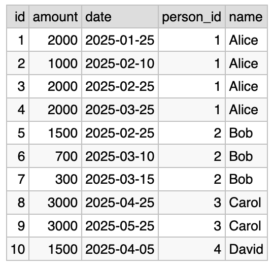
Let’s run a very simple query that shows list of payments, and the information about the employee:
SELECT payments.id, payments.amount, payments.date,
       people.id AS person_id, people.name
FROM payments LEFT JOIN people ON payments.employee_id = people.id
Result:
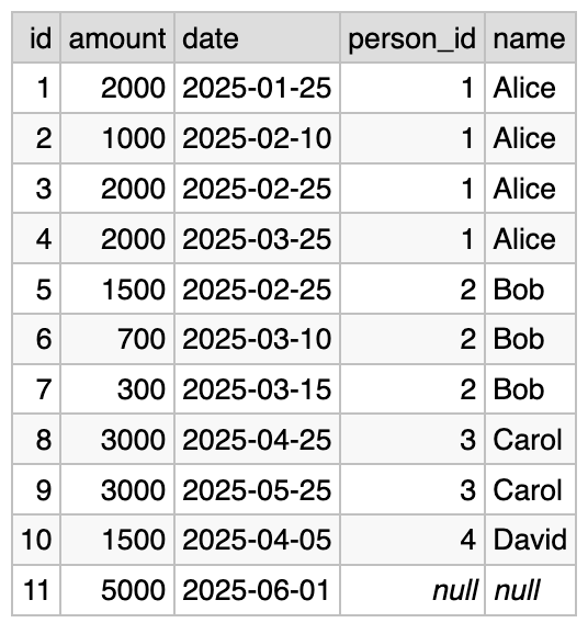
Roughly speaking, for each row in payments we look up a
corresponding row in the people table, using the value of
payments.employee_id.
people.id is a primary key, so we know that there is either one
corresponding row, or none at all. The latter case can happen if
payments.employee_id is NULL. If no record is found, then
people.id and people.name would be NULL, as can be seen in the
last result row.
We have 11 payments and we’re going to have 11 output rows; with filtering, we could have fewer rows, but we’ll never have more than that.
When the primary key is on the right side of equals sign in the ON condition, we call this “the N:1 case”.
N:1, 1:N, and M:N cases
We introduce the idea of three different cases when joining two tables:
- N:1 (this one is the best);
- 1:N;
- M:N;
How to find out which of the cases is that? We need to look at:
- first table:
payments; - second table:
people; - the ON condition:
ON payments.employee_id = people.id;
Now we need to ask several questions:
- for each row in the first table, how many rows in the second table could match our ON condition?
- if only one or zero, then our case is ?:1;
- if it could be many rows, then our case is ?:N;
- for each row in the second table, how many rows in the first table could match our ON condition?
- if only one or zero, then our case is 1:?;
- if it could be many rows, then our case is N:?;
Combining both halves, we would get one of “N:1”, “1:N”, or “M:N”. This is a very important information about your query, we’ll be using it consistently.
Let’s look again at our specific example. Given our ON condition:
-
for each row in the
paymentstable, only one row from thepeopletable could match (becausepeople.idis a primary key); -
for each row in the
persontable, many rows from thepaymentstable could match.
This is N:1. As we said before, it’s the best case.
It is very performant: joining on person ID requires only a primary key lookup. Primary key lookup is the most performant data querying operation imaginable.
Here is a surprising suggestion: maybe all of your LEFT JOINs need to be N:1, unless there is a good reason.
This is a rather bold statement, but let’s look at the 1:N case of LEFT JOIN and see that it’s so different from N:1 in all possible ways. Also, later in this chapter we’ll look into M:N case.
SQL may be too permissive
Due to historical reasons, SQL is very permissive. If your query is syntactically correct, the database is going to try and execute your query. It will go out of its way to execute your query, and you will never receive a pushback.
In this text we’re going to discuss several cases where the database lets you do something that you probably did not intend to do. Particularly:
- 1:N case of LEFT JOIN has a weird semantics;
- anything except for ID equality in ON condition is a potential mistake;
- foreign key definitions are ignored for JOINs: this lets you write syntactically correct but meaningless query;
- chained LEFT JOINs can lead to surprising performance degradation (5-6 or more orders of magnitude) that is not solved by indexes;
All those scenarios will sometimes bite you. Beginners would be especially vulnerable to that lack of guardrails, so in this article we give two strong suggestions for avoiding common query problems:
- always use ID equality comparison in ON condition;
- always use N:1 case of LEFT JOIN (primary key on the right);
But again, continue reading for more rationale behind those suggestions.
LEFT JOIN: 1:N case
Let’s take a query from the “N:1 case” section and swap the joined tables around:
SELECT people.id, people.name,
       payments.id AS payment_id, payments.amount, payments.date
FROM people LEFT JOIN payments ON people.id = payments.employee_id
Result:
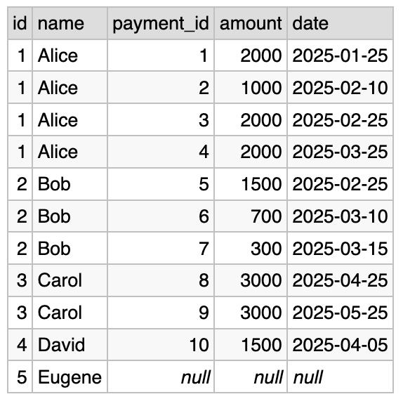
For readability, we also swapped the order of fields in the ON condition, and rearranged the list of columns in SELECT.
This query is syntactically correct. It is well-defined: anybody who knows SQL can easily understand what this query will return. Let’s see why we think that this type of query makes no particular sense.
Roughly speaking, for each row in people we query the
payments table, using the value of people.id. There could be any
number of payments corresponding to each person: zero, one or more.
If there is at least one payment, then there would be the same number
of result rows. However, if there are no payments then we’re going to
emit exactly one row, with the values of “payments.id”,
“payments.amount” and “payments.date” set to NULL.
The last sentence is what makes this case (we call it 1:N) so weird. This logic (NULL if no rows in the right table) works perfectly in the N:1 case, but let’s think about what we have here.
Is it one or another?
Do we have a list of payments here, or a list of people? Actually, we have something in between, depending on the data distribution. Here are three options:
1/ if it so happens that each person has at least one payment, then we’re going to have a list of payments, it makes sense;
2/ if one or more people has no payments (because they just joined the company), then we’re going to have a list of payments AND weird rows that are just record about a person; this makes less sense;
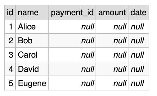
3/ imagine that the table of payments is empty (because our company was just established, and never had the chance to pay anyone). In this case, the result of our query would be basically a list of people. Here is how it looks like with empty list of payments:
Frankly, I know no other widely-used API that would return this sort of mixed results, except for this case. You can probably find some, because our industry has limitless imagination, but would you call such an API a well-designed API?
Forget SQL for a moment, how would you design a better result? You can return two lists: one is a list of payments, like we did in the N:1 case; another is a list of people who were never paid.
Fun fact: you can do that in SQL too, you just need to do two queries. First query we saw in a previous section, the second query would look something like (several variations are possible):
SELECT id, name
FROM people
WHERE id NOT IN (SELECT employee_id FROM payments);
So, we’re in a difficult situation here: this is, of course, one of the most basic SQL queries, it works in literally every database built in the past decades. Yet it’s not clear why this case even needed to be supported. I mean, you can certainly explain the chain of thought that happened around 40 years ago that has led us here, but this explanation does not make this case sensible and logical from the practical point of view.
See also the section about Venn diagrams below.
So what’s the practical outcome here? First, you must understand how LEFT JOIN works in a general case and in specific cases, that goes without saying. Everyone would expect you to understand it, it’s how databases work, it’s a completely non-controversial knowledge, it is what it is.
At the same time, notice when you attempt to use 1:N LEFT JOIN in one of your queries, and ask yourself if this is what you really need to do. There is a high chance that your query would be better written as N:1 LEFT JOIN, or as an INNER JOIN (see below).
However, see also the section about LEFT JOIN and GROUP BY below, where a possible exception from this rule is discussed.
Why you should only use ID equality
Note: this section talks about INNER JOIN (covered below in the “INNER JOIN” chapter), particularly its excessive flexibility. However, this is one of the most important ideas of this text, worth presenting early. You may want to revisit this subsection after reading about INNER JOIN.
In this guide we strongly suggest that you use only ID equality in ON condition. All other filtering must go into WHERE. This applies to both LEFT JOIN and INNER JOIN. For the latter, this is technically not necessary, but we’ll present a scenario where this can become a gotcha.
If your query does not follow this rule and you are getting unexpected results, the first recommendation would be to rewrite your query and see if it works.
Let’s look first at an example of a simple query that works in a confusing way. Suppose that we want to get a list of payments less than some amount. This is basically a N:1 LEFT JOIN plus an extra filtering condition. Let’s knowingly violate the “ID equality only” rule and see what happens:
SELECT payments.id, payments.amount, payments.date,
       people.id AS person_id, people.name
FROM payments LEFT JOIN people
  -- this is incorrect condition
  ON payments.employee_id = people.id AND payments.amount < 1000
Here is the result:
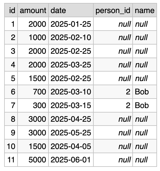
Wow, what happened to our “AND payments.amount < 1000”? To understand why this happens, you need to look at the fully general LEFT JOIN algorithm below and see that this is exactly how it’s supposed to work.
Here, this part of a condition is used for matching, and not for filtering. And due to the way LEFT JOIN works, when the matching function returns false, we still output the rows from the left table.
To fix this, you just need to follow the advice and move the filtering condition into WHERE clause:
SELECT payments.id, payments.amount, payments.date,
       people.id AS person_id, people.name
FROM payments LEFT JOIN people
  ON payments.employee_id = people.id
WHERE payments.amount < 1000

Second part of the potential gotcha is that for INNER JOIN this does not apply: ON and WHERE conditions in INNER JOIN are fully interchangeable (see the section below).
But you still have to keep this discipline of only using ID equality in ON condition, even for INNER JOIN! This is because as you work on query, you can sometimes switch back and forth between LEFT and INNER JOIN. So it happens like this:
- you have a sloppy ON condition in INNER JOIN;
- you change to LEFT JOIN: for example, you want to include even payments that are not sent to employees;
- your ON condition becomes incorrect;
In this example everything is clearly visible, and the query is as simple as possible, you will quickly find the mistake. But if you have a subquery or a CTE it may be much more tricky.
So, keep some discipline and use only ID equality comparison in ON condition. Unfortunately, this is one of the places where SQL does not prevent you from doing the potentially incorrect thing.
Self-join
So, here is a simple problem: show a list of people with the name of their manager. Remember that some people, like Alice, don’t have managers.
In our people table, there are two columns that contain IDs: “id” and “manager_id”. They both contain IDs of people, and that means that we can write a JOIN based on those two IDs. Those two columns are in the same table, but that’s fine, it’s just a self-join.
One thing that we must do when writing a self-join query is to remove
name ambiguity by aliasing one or both tables. This is done using the
“AS” keyword.
Also, we need to make sure that we choose the N:1 JOIN. Let’s talk this through:
- each employee has only one employee as manager, or none; (N:1)
- each employee can be a manager of several employees; (1:N)
Here is the query:
SELECT subordinates.id, subordinates.name, managers.id, managers.name
FROM people AS subordinates LEFT JOIN people AS managers
     ON subordinates.manager_id = managers.id
And here is the result:
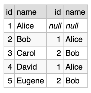
As you can see, Alice does not have a manager. Bob has Alice as manager, and so on.
Let’s look at the query. We joined a table to itself, and we specified table aliases for both sides of JOIN: “subordinates” and “managers”.
There is nothing complicated about self-joins, really. You should use the N:1 case, and you should alias the table names. Self-joins are mostly used when there is some sort of hierarchy, like in manager-subordinate relationships. Here are some other possible self-join scenarios that come to mind:
- manager/subordinates is an archetypal example;
- nested folders like in Google Docs: a folder can contain other folders;
- referred accounts: if your website allows to refer people for signup, you can have a hierarchy of sign-ups;
- threaded comments, like on Reddit: you can reply directly to the post, or to another comment;
If you want to get acquainted with self-join, try implementing one of the scenarios listed here, add some test data and try running queries. All self-join queries are very similar; only the table names, aliases and column names would be different.
One advanced case not covered here is called recursive joins. Not all databases support it, and you have to read about that elsewhere.
Fully general LEFT JOIN algorithm
So far we’ve discussed three restricted cases of ON condition:
- ID equality comparison, N:1 case;
- ID equality comparison, 1:N case;
- ID equality comparison + some other condition;
But LEFT JOIN was introduced as a fully general algebraic operation half a century ago, and it is implemented as a fully general algebraic operation in all SQL databases.
In this text we will deviate again from the commonly-presented declarative approach to LEFT JOIN. Instead we present an imperative approach to explaining how LEFT JOIN works in the most general case.
(See the corresponding section below for the discussion of declarative vs imperative approaches.)
Anyway, here is the:
Generalized LEFT JOIN algorithm
Suppose that the first table looks like:
(id1, col_a, col_b, …).
And the second table looks like:
(id2, col_t, col_x, …).
For each row of the first table we do the following:
-
Select all the rows in the second table such that ON condition returns true;
-
If one or more rows are found:
-
append the values from the first table row to each of the rows found:
(id1, col_a, col_b, …, id2, col_t, col_x, …). -
Add each of the found rows to the output dataset;
-
-
If no rows were found in the second table, add exactly one row anyway containing first table row values and as many NULLs as needed:
(id1, col_a, col_b, …, NULL, NULL, NULL, …).
End.
Only after this main part of the algorithm is finished, the WHERE condition could be applied to filter out some of the rows.
The main part of this algorithm works in a peculiar way. Notice the following:
-
the output contains at least as many rows as in the first table;
-
only if the first table is empty, the output would be empty;
-
the output could contain more rows than in the first table;
Here this algorithm is abstractly defined as a nested loop, but the real query engine processes LEFT JOINs in a variety of optimized ways depending on ON condition and table schemas.
This is why the N:1 case is so important: it is the most efficient to implement in practice: basically there is no inner loop. However, do not worry about optimization and execution plan here: our goal is to learn the abstract definition.
See also
In the general case there is no restriction on what ON condition does. In real-world queries it almost always compares two IDs from two tables. But there are some exotic ON conditions such as “always true” and “always false” that we discuss later in this text.
We’ll discuss the declarative approach to understanding LEFT JOIN below.
Also, we need to discuss why “returns all rows” wording is misleading. Unfortunately, it is very commonly seen on the internet and in LLM outputs, so you need to understand how this wording may hurt your understanding. We, of course, do not use this wording here. See the corresponding section below.
Things to remember, pt. 1
A brief summary of things I want you to remember from this:
-
use only ID equality comparison in ON condition, everything else goes to WHERE;
-
learn LEFT JOIN first, even though traditionally people begin with INNER JOIN;
-
LEFT JOIN is better understood as three distinct subcases:
-
N:1 case, ID equality only: the most useful and most performant;
-
1:N case, ID equality only: quite weird, and you can avoid it;
-
fully general case with arbitrary ON conditions;
-
-
N:1 case means that there is a primary key to the right of the equals sign;
-
SQL is too permissive and does not protect you from simple mistakes: performance issues and unexpected results may occur;
-
you need to understand the entirety of LEFT JOIN semantics so that you can read and modify queries written by other people;
-
fully-general LEFT JOIN algorithm is better presented as simple imperative nested loop;
-
if you follow advice presented here, you will prevent many typical mistakes and make your queries faster and more readable;
“Database Design Book” (2025)
Learn how to get from business requirements to a database schema
If this post was useful, you may find this book useful too.
Table of contents and sample chapters
Book length: 145 pages, ~32.000 words. Available in both PDF and in EPUB format.
Continue with INNER JOIN
LEFT JOIN and INNER JOIN are closely related. It’s possible to express one in terms of another, but we believe that this is not useful for understanding.
That’s why we treat INNER JOIN as a separate concept.
Use canonical syntax
For INNER JOIN we’re going to use a standard syntax:
SELECT tableA.*, tableB.*
FROM tableA INNER JOIN tableB ON tableA.id = tableB.another_id
WHERE ...
That’s virtually the same standard syntax as in LEFT JOIN, only one word is different.
Historically, INNER JOIN has a variety of legacy syntaxes that are widely supported. We’ll discuss them later in a separate section. You need to know legacy syntax to understand queries written by other people.
Use only ID equality comparison
When writing INNER JOIN queries, we also insist on using only ID equality comparison in ON conditions, same as for LEFT JOIN.
In the latter section we show that technically it is not necessary. Yet, following this advice prevents the possibility of coding mistakes that may arise from changing between INNER JOIN and LEFT JOIN.
N:1 case of INNER JOIN
Let’s modify the query from “N:1 case of LEFT JOIN” section, changing it to INNER JOIN:
SELECT payments.id, payments.amount, payments.date,
       people.id AS person_id, people.name
FROM payments INNER JOIN people ON payments.employee_id = people.id
Here is the result:
Note that instead of 11 result rows we now have only 10. The last
row was filtered out because payments.employee_id has the value of
NULL, which has no corresponding row in the people table.
We’ll discuss the fully general INNER JOIN algorithm shortly, but let’s see how the N:1 case works.
Roughly speaking, for each row in payments we’re going to look up a corresponding row in the people table, using the value of payments.employee_id. We know that there is either one record, because people.id is a primary key, or there is no record at all, maybe because payments.employee_id is NULL. If an employee record is found, a row is added into the result dataset. Otherwise, this row of payments is skipped.
Implicit filtering
We call this behavior implicit filtering. The result contains only those payments that have a corresponding employee. Do you need it? It depends on what you want to see. If you want to have a list of employee payments you can use INNER JOIN; if you want to have the entire list of payments you can use LEFT JOIN.
Let’s look at the explicit filtering too. In principle, it’s possible to achieve the same result as above (for the N:1 case) by using LEFT JOIN and adding a WHERE condition:
SELECT payments.id, payments.amount, payments.date,
       people.id AS person_id, people.name
FROM payments LEFT JOIN people ON payments.employee_id = people.id
WHERE people.id IS NOT NULL
We’ll get the same 10 rows. However, it’s better to write the minimal variant of that query because it is shorter and more readable.
Also, using INNER JOIN may be better handled by your database query engine because the behaviour it requires is much simpler.
Is it always possible to express INNER JOIN via LEFT JOIN and WHERE … IS NOT NULL? Let’s discuss that in a separate section.
Fully general INNER JOIN algorithm
Having discussed the N:1 case, we can jump straight to the fully general case. It is much easier than LEFT JOIN.
We again present it in a way that deviates from how it is presented in common teaching materials. We define it in an imperative way first. For INNER JOIN it makes sense to present the declarative way too, because it is more enlightening.
Anyway, here is the
Generalized INNER JOIN algorithm
For each row of the first table we do the following:
- For each row of the second table we evaluate the ON condition. If it returns true, we add a row to the output. Data from all columns of both tables is available for output.
End.
This is abstractly defined as a nested loop, but the real query engine processes INNER JOINs in a variety of optimized ways depending on ON condition and table schemas. This is why the N:1 case is so important: it is the most efficient to implement in practice: basically there is no inner loop. Do not worry about optimization and execution plan here: our goal is to learn the abstract definition. (This paragraph was copy-pasted from the LEFT JOIN chapter with only one word changed.)
Now let’s look at the declarative approach to INNER JOIN.
INNER JOIN is filtered Cartesian product
First we need to explain what a Cartesian product is. Imagine two
tables called “foo” and “bar” (meaningless names are chosen
deliberately). Those tables are very narrow, each containing only one
column called “val”. “foo” contains five rows with the following
values: “A”, “B”, “C”, “D”, and “E”. “bar” contains three
rows with the following values: 1, 2, 3.
The Cartesian product of two tables is a list of all possible pairs of rows taken from each of the tables. In our example, there are 3 x 5 = 15 such pairs.
foo x bar |
|
|---|---|
(foo.val) |
(bar.val) |
| (“A”) | (1) |
| (“A”) | (2) |
| (“A”) | (3) |
| (“B”) | (1) |
| (“B”) | (2) |
| (“B”) | (3) |
| (“C”) | (1) |
| (“C”) | (2) |
| (“C”) | (3) |
| (“D”) | (1) |
| (“D”) | (2) |
| (“D”) | (3) |
| (“E”) | (1) |
| (“E”) | (2) |
| (“E”) | (3) |
You can also represent this in a different way if it helps with understanding:
| →: (bar.val) ↓: (foo.val) |
(1) | (2) | (3) |
|---|---|---|---|
| (“A”) | (“A”), (1) | (“A”), (2) | (“A”), (3) |
| (“B”) | (“B”), (1) | (“B”), (2) | (“B”), (3) |
| (“C”) | (“C”), (1) | (“C”), (2) | (“C”), (3) |
| (“D”) | (“D”), (1) | (“D”), (2) | (“D”), (3) |
| (“E”) | (“E”), (1) | (“E”), (2) | (“E”), (3) |
The vertical format is closer to how the database tables are represented. Rectangular format helps you see that there is a multiplication involved.
So, the Cartesian product is a full list of possible pairs. INNER JOIN takes this full list, and leaves only those pairs where ON condition returns true. (After that, we’ll also additionally filter by the WHERE condition.)
How can it be used in practice? Let’s get back to that question a bit later.
INNER JOIN syntax is very permissive
First, you can swap the order of tables in INNER JOIN, and the result will be exactly the same.
SELECT payments.id, payments.amount, payments.date,
       people.id AS person_id, people.name
FROM payments INNER JOIN people ON payments.employee_id = people.id
could be written as
SELECT payments.id, payments.amount, payments.date,
       people.id AS person_id, people.name
FROM people INNER JOIN payments ON people.id = payments.employee_id
Second, the conditions in ON and WHERE clauses are completely interchangeable. They are logically AND’ed together, so the result does not change. Let’s take a fragment of our query, written in a canonical form (ID equality comparison), and add some WHERE condition:
SELECT ...
FROM payments INNER JOIN people ON payments.employee_id = people.id
WHERE payments.amount > 1000
Technically you can write this query in three more ways:
- move all conditions to ON:
FROM payments INNER JOIN people
     ON payments.employee_id = people.id AND payments.amount > 1000
- swap ON and WHERE conditions — do not do this, it’s horrible:
FROM payments INNER JOIN people ON payments.amount > 1000
WHERE payments.employee_id = people.id
- move all conditions to WHERE; we have to have something in ON, so we used
1=1, an “always true” condition — also horrible but fun:
FROM payments INNER JOIN people ON 1=1
WHERE payments.employee_id = people.id AND payments.amount > 1000
Additionally, of course, you can swap the order of tables as mentioned above, and the order of AND subclauses.
This flexibility becomes a problem when you want to change the query from INNER JOIN to LEFT JOIN. This occasionally happens when you write long complicated queries, and that’s why we insist on keeping the discipline of writing both kinds of JOINs: so that they could be trivially changed from one to another.
Reminder:
- ON condition: ID equality comparison only;
- everything else goes to WHERE;
- order of tables is N:1, avoid 1:N;
Historical syntax for INNER JOIN
Let’s look again at the canonical syntax for INNER JOIN:
SELECT payments.id, payments.amount, payments.date,
       people.id AS person_id, people.name
FROM payments INNER JOIN people ON payments.employee_id = people.id
You need to be aware of several variations of INNER JOIN syntax, because you will see them in queries written by other people, particularly in teaching material. We’ll briefly cover the most important variations.
First, you can omit the “INNER” keyword and just use “JOIN”.
Second, you can write table names separated by commas, without any JOIN keyword:
SELECT payments.id, payments.amount, payments.date,
       people.id AS person_id, people.name
FROM payments, people
WHERE payments.employee_id = people.id
Don’t use this.
Third, CROSS JOIN is also equivalent to INNER JOIN:
SELECT payments.id, payments.amount, payments.date,
       people.id AS person_id, people.name
FROM payments CROSS JOIN people
WHERE payments.employee_id = people.id
There are also even less commonly used syntaxes.
SELECT *
FROM table_a INNER JOIN table_b USING (id)
would be the same as “ON table_a.id = table_b.id”. Don’t use this.
Don’t use NATURAL JOIN either, it’s even more weird, there is
nothing natural in it.
Cartesian product in practice
So, we discussed that INNER JOIN is just a Cartesian product with filtering. Abstractly speaking, we take each possible pair of rows from both tables, and then filter out some of them.
In most practical queries, this process is heavily optimized, especially if you use only ID equality comparison in your ON conditions. In this case the rows are not multiplied, or, technically speaking, they are “multiplied by 1”.
There are some rare examples where actual Cartesian product behaviour may be useful. Imagine a habit tracker. Suppose that you have a list of dates and a list of habits. List of dates is: 2026-01-01, 2026-01-02, 2026-01-03, …, 2026-01-07. List of habits is: a) journaling; b) yoga; c) meditation; d) go outside.
What happens if you “multiply” the list of dates by the list of
habits? You will have 28 rows (7 days times 4 habits) that contain
something like a checklist of habits over the week. “Did you do
journaling on Jan 1st? Did you do yoga on Jan 2nd?” etc. Here is
this toy example:
https://dbfiddle.uk/94Lxff0W. See the
data definition, then an INNER JOIN ON 1=1, then a count (it shows
28 rows, as expected).
This is not a very interesting use case, but you need to be aware of the possibility of doing something like that. This behavior of the Cartesian product is embedded deep into the way SQL works technically.
(If you know a good use case for a true Cartesian product, drop me a line.)
What’s more important is that you must understand the Cartesian behavior so that you could recognize it if you make a mistake, or if you have to debug a query. If you accidentally use the incorrect ON condition one of your subqueries may return way too many rows than intended. This is especially possible if comma-separated syntax is used, and there are more than two tables.
CROSS JOIN is equivalent to INNER JOIN
There is another weird detail about how SQL is traditionally presented. For some reason, Cartesian behavior of INNER JOIN is often not acknowledged in teaching texts.
For example, many tutorials make a distinction between INNER JOIN and CROSS JOIN. They spend a lot of time teaching INNER JOIN but somehow omit mentioning the basic fact that they are identical. Towards the end of the tutorial they go on discussing CROSS JOIN without mentioning that it’s just a tiny variation of INNER JOIN, just another historical syntax.
Proof: you can generate a full Cartesian product of two tables using INNER JOIN together with “always-true” ON condition:
SELECT *
FROM dates INNER JOIN habits ON 1 = 1
Equivalent CROSS JOIN syntax:
SELECT *
FROM dates CROSS JOIN habits
Another thing that we need to discuss is a problem with the “returns all rows” wording, which also contributes to conceptual misunderstanding. See a section on that below.
Things to remember, pt. 2
- INNER JOIN is symmetrical: order of tables technically does not matter;
- INNER JOIN is not strict about what goes to ON and what goes to WHERE;
- however, if you write INNER JOIN in a disciplined way, you can trivially change to LEFT JOIN;
- use only ID equality comparison in ON condition, everything else goes to WHERE;
- the government does not want you to know that INNER JOIN is a Cartesian product, aka CROSS JOIN;
- you need to learn half a dozen of historical syntaxes of INNER JOIN to be able to read other people’s queries; do not use them yourself;
- N:1 case of INNER JOIN is the most performant;
- N:1 case of INNER JOIN provides implicit filtering, which is perfect if you need it;
Common bad explanations
Venn diagrams is a bad explanation
You’ve probably seen some Venn diagrams that are supposed to “explain” SQL JOINs. Unfortunately, they are completely useless because they do not explain anything.
Let’s discuss what is wrong with Venn diagrams in this context.
Problem 1. What does the dot mean?
First, what is a Venn diagram? Suppose that we want to show that a) some students learn SQL, b) some learn Java and c) some learn both of those languages. This is a perfect use case of the Venn diagram:
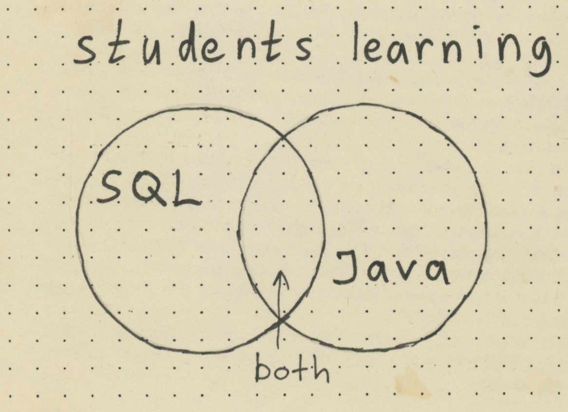
The circles correspond to groups of people, and some people are only learning SQL, some are learning only Java, and some are learning both. Now we can discuss all three groups, and everything is pretty clear. Each dot represents a person.
Going back to SQL JOINs diagram, here is a typical example:
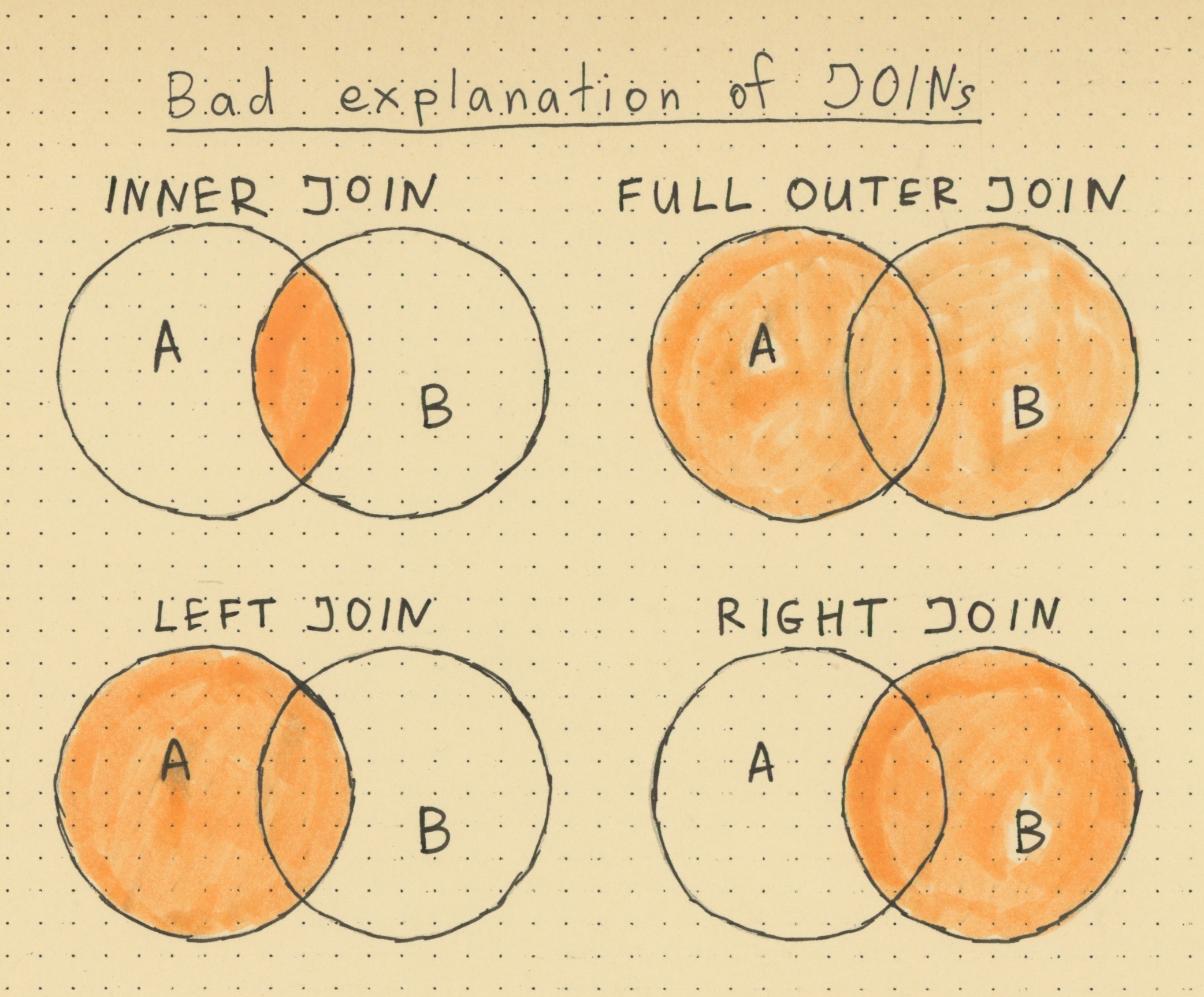
Note that such diagrams always use “A” and “B”, thus hiding the problem. What is “A” and what is “B”? Let’s use our table names instead of meaningless labels:

What is going on here? What is a dot in this diagram? A dot could not be a payment, because there are dots outside of the “payments” circle. A dot could not be a person, because there are dots outside of the “people” circle. What does the dot in the intersection supposed to mean?
Problem 2. Multiplicative behavior is not shown
If you look at the Venn diagram, even if you provide meaningful labels, the multiplicative behavior is not represented graphically. This I believe is a huge problem, together with a typical “returns all rows” wording (see below).
Venn diagrams here are very informally supposed to correspond to rows. So, every dot is a row in some table, right? Unfortunately, this nudges us away from understanding the multiplicative behavior of JOINs.
One extra problem is that Venn diagrams were originally created to illustrate basic concepts from set theory. And the relational model is also based on set theory. But the Venn diagram, if applied here, is not an accurate representation of how JOINs work.
Problem 3. RIGHT JOIN
RIGHT JOIN is a waste of words and pixels. Giving it 25% of picture size is extremely wasteful. (See below for more details).
Conclusion
Considering all this, it’s clear that Venn diagrams are disappointingly low-content for the purpose of teaching SQL JOINs. Even if you consider them some sort of mnemonics: what does it help you to remember? If the spot of color is on the left then it’s LEFT JOIN, if the spot of color is in the middle then it’s INNER JOIN, and so on. Where is the value in that?
RIGHT JOIN is a waste of words and pixels
All you need to know about RIGHT JOIN:
b RIGHT JOIN ais syntactically equivalent toa LEFT JOIN b.
That’s it. You virtually never see RIGHT JOIN in real queries, except as a sort of a joke.
The only place where you keep seeing a lot of RIGHT JOINs is in the low-effort basic SQL tutorials that get copy-pasted over and over and over again. They often dedicate the same amount of words and pixels to LEFT and RIGHT JOINs without any benefit for the reader. Avoid those.
“Returns all rows” is misleading
Let’s google “how left join works” and see what the first few results tell us.
W3schools.com (the top snippet): “The LEFT JOIN command returns all rows from the left table, and the matching rows from the right table.”
Learnsql.com: “LEFT JOIN, […] returns all records from the left (first) table and the matched records from the right (second) table.”
TutorialsPoint.com: “Left (Outer) Join: Retrieves all the records from the first table, Matching records from the second table and NULL values in the unmatched rows.”
This is just three examples, but there are many more. I believe that “all rows” wording is misleading and should be avoided in teaching materials.
For me “all records [from the left table]” means that the result dataset will contain no more than the number of records in the left table. We know that this is not true in the general case: LEFT JOIN can return multiple of that.
If I give you 100 apples and tell you “give me back all the apples that have no spots”, I’d be extremely surprised if you returned 250 apples.
Interestingly, this wording would be perfectly accurate if we would only allow N:1 case of JOIN. There would have been no multiplication, and we would expect to return no more than the number of records in the left table. But this is not how it works in reality.
(So far I could not find a satisfactory summary of fully general LEFT JOIN algorithm.)
“Database Design Book” (2025)
Learn how to get from business requirements to a database schema
If this post was useful, you may find this book useful too.
Table of contents and sample chapters
Book length: 145 pages, ~32.000 words. Available in both PDF and in EPUB format.
Extra chapters
LEFT JOIN + GROUP BY
Let’s investigate the 1:N case of LEFT JOIN together with GROUP BY.
Suppose that we want to find out how much we paid to each of our employees, including those who haven’t been paid yet.
This is a simple GROUP BY query:
SELECT people.id,
       COUNT(payments.id) AS cnt,
       SUM(payments.amount) AS total
FROM people LEFT JOIN payments ON people.id = payments.employee_id
GROUP BY people.id
For our dataset, this would return the following:
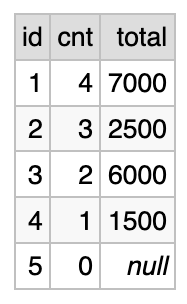
For each person we show: their ID, the number of payments that were made (“cnt” column), and the total amount of payments.
The results include people who did not have any payments, such as Eugene (ID=5). We see cnt=0 in the last line, and total=NULL.
This simple example actually brings a lot of questions!
First, note that we had to use COUNT(payments.id), and not
COUNT(*) (that would have shown 1 instead of 0). This is because
COUNT() implicitly counts only non-null values.
Second, SUM(payments.amount) returns NULL. Maybe we would have
preferred to see 0 here. To get 0 we have to use something like
COALESCE(SUM(payments.amount), 0). COALESCE() returns the first
non-NULL argument, so in this example it essentially replaces NULL
with 0.
But here is the main thing. This query seems to be a perfect application of 1:N case of LEFT JOIN. It shows all that we want: most importantly, the aggregate data for users who did not have corresponding rows in the payments table. The execution plan is pretty efficient. Two small points that we noted just require a bit of care.
Unfortunately, only this simplest two-table case is guaranteed to be that predictable. If you try to add more statistics from a different table: say, a number of tickets closed, you immediately run into a potential problem.
Chaining LEFT JOIN with one more table
Let’s create another table called “tickets”, and insert just the three rows for Carol, pretending that she has three tickets assigned.
CREATE TABLE tickets (
  id INTEGER NOT NULL PRIMARY KEY,
  description VARCHAR(255) NOT NULL,
  assigned_to INTEGER NOT NULL
);

CREATE INDEX ndx_tickets_assgn_to ON tickets(assigned_to);

INSERT INTO tickets (id, description, assigned_to) VALUES
  (1000, 'Fix frontend bug', 3),
  (1001, 'Improve backend feature', 3),
  (1002, 'Document our database', 3);
The following query seems to be just marginally more complex (scroll down to the bottom in this playground URL: https://dbfiddle.uk/4jvpkjHa):
SELECT people.id,
       COUNT(payments.id) AS cnt,
       SUM(payments.amount) AS total,
       COUNT(tickets.id) AS ticket_cnt
FROM people LEFT JOIN payments ON people.id = payments.employee_id
            LEFT JOIN tickets ON people.id = tickets.assigned_to
GROUP BY people.id
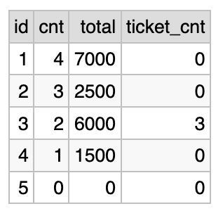
Unfortunately, this query is broken in several different ways. Some can be fixed, but some require a completely different approach, explained below. Let’s take a look at the results (together with the previous version):
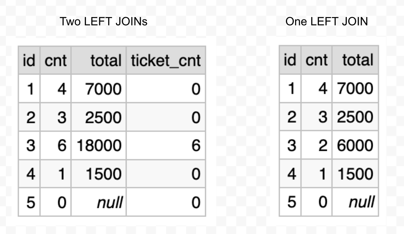
Look at the line that corresponds to ID=3. You see that the number of payments is now 6 instead of 2, and the total amount of payments is 18000 instead of 6000. Both numbers were multiplied x3, which suspiciously matches the number of tickets assigned to Carol.
But wait, there is more: the number of tickets is also incorrect: it’s 6 and not the expected 3. The number is multiplied x2, which suspiciously matches the number of payments made to Carol.
This is what people call “overcounting”.
Understanding the problem of overcounting
Overcounting manifests because the 1:N case of LEFT JOIN introduces multiplication, as we discussed above. Aggregation functions such as COUNT() or SUM() are computed after the underlying dataset is constructed, and the underlying dataset contains lots of duplicates.
In principle, you could fix the problem partially by adding DISTINCT (see the playground at https://dbfiddle.uk/fio49Qty):
SELECT people.id,
       COUNT(DISTINCT payments.id) AS cnt,
       SUM(payments.amount) AS total,
       COUNT(DISTINCT tickets.id) AS ticket_cnt
FROM people LEFT JOIN payments ON people.id = payments.employee_id
            LEFT JOIN tickets ON people.id = tickets.assigned_to
GROUP BY people.id
And the counts are now fixed:
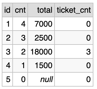
Unfortunately, you cannot fix the SUM of payments this way. If you’d use DISTINCT it would take only payment amounts that are different from one other. But it is normal to have several payments with identical amounts. A different approach is needed.
Performance problems with LEFT JOIN chaining
But in many applications, you only need counts (no sums). Could you just add DISTINCT everywhere, do not use SUM() and call it a day? Unfortunately, there may be another problem on the horizon.
You may be lucky and the “fixed” query would run as quickly as the first one, or at least in the acceptable time. But you may also be unlucky and it will take a lot longer: like, 10000 times more (four orders of magnitude), and I am not even exaggerating. In my testing on a real-world database the first query runs in 0.05 seconds, while the second one takes 12 minutes (14500x slowdown).
Whether it would happen or not, depends on several factors. First, it depends on the capabilities of your database server. Second, it depends on specific data distribution in your tables.
Particularly, such a query may work with acceptable performance on smaller datasets, and then slow down drastically as the dataset grows, or data distribution pattern changes.
Note that this problem has nothing to do with indexes, and you may not be able to solve it by looking at the execution plan. The actual reason is how the underlying dataset is generated and then aggregated.
Systematic design of multi-join GROUP BY queries
Earlier this year I wrote a very long two-part treatise on writing complicating SQL queries based on JOINs and GROUP BY aggregations.
Part 1: “Systematic design of multi-join GROUP BY queries” https://kb.databasedesignbook.com/posts/systematic-design-of-join-queries/ (~5400 words). Explains a systematic approach to building complicated queries that takes into account all the problems that we’ve discussed in this text, starting from the beginning. Shows how to optimize queries for modern distributed environments, enabling pipeline-based processing of complicated analytical queries.
Part 2: “Multi-join queries design: investigation” https://minimalmodeling.substack.com/p/multi-join-queries-design-investigation (~3500 words). Investigates the performance degradation problem, introduces the idea of “underlying dataset”, shows that indexes are not a problem here. Introduces the idea of query design, complementary but distinct from database design.
The approach explained in those two texts systematically uses N:1 case of LEFT JOIN. Among other things, if you write complicated queries in such a way, they will have consistent performance, independent of data distribution and less dependent on database capabilities. Also, it enables further higher-level query optimizations.
The guide that you are reading now is written as a sort of prequel to the first two parts. It is intended to help you nail the correct mental model before you can safely tackle complicated scenarios that you may encounter in production databases.
Note that commonly used LLMs consistently get confused about that topic. In some cases they will proudly announce that they just wrote you a correct SQL query that avoids double-counting, but for a different case they will get back to writing a knee-jerk LEFT JOIN chaining version. They certainly know about the overcounting problem, but they don’t always use that knowledge.
Correct approach to multiple LEFT JOINs
As a simple illustration of the systematic approach presented in the previous section, let’s see how our three-table query should look. There are three roughly equivalent approaches: subqueries, CTEs and correlated subqueries. CTE may be the most readable (playground: https://dbfiddle.uk/_BoxwX6C):
WITH payments_agg AS (
  SELECT employee_id, COUNT(*) AS cnt, SUM(amount) AS total
  FROM payments
  GROUP BY employee_id
),

tickets_agg AS (
  SELECT assigned_to, COUNT(*) AS cnt
  FROM tickets
  GROUP BY assigned_to
)

SELECT people.id,
       COALESCE(payments_agg.cnt, 0) AS cnt,
       COALESCE(payments_agg.total, 0) AS total,
       COALESCE(tickets_agg.cnt, 0) AS ticket_cnt
FROM people LEFT JOIN payments_agg ON people.id = payments_agg.employee_id
            LEFT JOIN tickets_agg ON people.id = tickets_agg.assigned_to
ORDER BY people.id
Output:
This approach and its variations are extensively analyzed in the posts linked above. We won’t go deeper here.
Conclusion
Here are the key takeaways of this guide:
-
stick to disciplined patterns of using JOIN: SQL is too permissive for your own good;
-
use only ID equality in ON condition: all other filtering belongs to WHERE;
-
strongly prefer the N:1 join pattern (unique key on the right side of JOIN): it is both less error-prone and more performant;
-
learn the full range of SQL variations: you need to be able to read all sorts of SQL queries and collaborate on them;
The approach presented here scales directly to much more complicated SQL queries.
Thanks for reading.
I’d be happy to hear your feedback:
Alexey Makhotkin
squadette@gmail.com.
“Database Design Book” (2025)
Learn how to get from business requirements to a database schema
If this post was useful, you may find this book useful too.
Table of contents and sample chapters
Book length: 145 pages, ~32.000 words. Available in both PDF and in EPUB format.